where \(\boldsymbol{\sigma}\) is a vector of tractions and rotational components, and \(\boldsymbol{\varepsilon}\) is a vector of strains obtained from displacement jumps smeared over the element length and rotational components.
Furthermore, \(\mathbf{D}_{\rm e}\) is the elastic stiffness matrix which is based on the elastic modulus of the lattice material \(E\), and a parameter \(a_1\) which is the ratio of the modulus of the shear and normal direction. There is the option to include a rotational stiffness. The model parameters are summarised in Table 73.
Table 73 Linear elastic material model for lattice elements – summary.
[talpha] Thermal strain expansion coefficient. Default is 0.
[calpha] Thermal displacement expansion coefficient. Default is 0.
e Young’s modulus of the lattice springs (normal stiffness). At least one of
e and em must be given; if e is omitted, it is set from
em (see nu).
[em] Macroscopic Young’s modulus of the continuum to be represented. Default is
e.
[nu] Poisson’s ratio (must be < 1). If given, the spring ratios are derived from
it following Griffiths and Mustoe (2001): \(a_1 = (1-3\nu)/(1+\nu)\). If em
is given without e, the spring modulus is scaled as \(E = E_{\rm m}/(1-\nu)\)
and \(a_2 = 1/(1+\nu)\), otherwise \(a_2 = 1\). Explicitly given a1 and
a2 take precedence.
[a1] ratio of shear and normal modulus. Default is 1.
[a2] ratio of rotational and normal modulus. Default is 1.
[bio] Biot’s coefficient used when the element is coupled to a lattice transport
problem (pressure acting on the mechanical response). Default is 0.
All lattice structural materials derived from the linear elastic lattice model accept two optional parameters, [randvars (ia)] and [randgen (ia)], which assign spatially varying values to selected material properties. randvars is a list of property identifiers and randgen is a list of the same length with the numbers of the functions (see the time function records in the OOFEM input manual) that generate them. When the material status of an integration point is created, each function is evaluated at the global coordinates of that point (variable x) and the result is stored as a multiplicative factor on the mean value of the corresponding property. A typical choice is an InterpolatingFunction reading a precomputed random field from a file.
The property identifiers that are currently queried are
1101 (eNormal_ID): factor on the spring modulus e, used by latticelinearelastic, latticedamage and latticeplastdam;
800 (e0_ID): factor on the strain threshold e0 of latticedamage;
806 (ft_strength): factor on the tensile strength ft of latticeplastdam;
807 (fc_strength): factor on the compressive strength fc of latticeplastdam.
The factor is limited to the range 0.1 to 10. Identifiers that a model does not query are silently ignored.
Example: latticedamage1d2400.e30.e9e0100.e-6wf40.e-6stype3randvars1800randgen12 scales e0 by the field generated by function 2.
Example: latticeplastdam1d0talpha0.e40.e9a10.175a21.ft6.5e6fc130.e6angle10.5angle20.5flow0.25wf1.53e-5ahard1.e-3iter100tol1.e-6randvars2806807randgen233 scales both ft and fc by the field generated by function 3, for example InterpolatingFunction3namefield.datdim3 (see lm/latticeplastdam3drandom.in).
This is a scalar damage material model used together with lattice elements.
It uses a scalar damage model, which results in a stress-strain law of the form
where \(\boldsymbol{\sigma}\) is a vector of tractions and rotational components, and \(\boldsymbol{\varepsilon}\) is a vector of strains obtained from displacement jumps smeared over the element length and rotational components.
Furthermore, \(\omega\) is the damage variable varying from 0 (undamaged) to 1 (fully damaged).
Also, \(\mathbf{D}_{\rm e}\) is the elastic stiffness matrix which is based on the elastic modulus of the lattice material \(E\), and a parameter \(a_1\) which is the ratio of the modulus of the shear and normal direction.
The strength envelope (onset of damage) is elliptic and determined by three parameters, \(f_{\rm t}\), \(f_{\rm q}\), and \(f_{\rm c}\). The evolution of the damage variable \(\omega\) is controlled by normal stress-normal crack opening law. The three possible laws are linear, bilinear, and exponential.
This simple damage material model for lattice elements has been used in many recent articles. For instance, the two-dimensional version has been used in [GraJir10]. An example of an application of the three-dimensional version of the model is found in [GraBol16].
A variant of the scalar damage lattice model for shell-type lattice analysis. It
works only with the lattice3d and lattice3dnl elements. It uses a
shell-specific equivalent-strain measure but is otherwise identical to the scalar
damage model; the input record and parameters are the same as for
latticedamage, using the keyword latticedamageshell.
This combined plasticity damage model for lattice elements has been developed to describe the failure process of geomaterials such as concrete and rock. The plasticity part is based on the effective stress and damage is evaluated by the plastic strain. The model was first introduced in [GraDav11] without hardening and then extended to hardening in [AthWheGra18].
where \(\boldsymbol{\sigma}\) is a vector of tractions and rotational components, \(\omega\) is the damage variable and \(\mathbf{D}_{\rm e}\) is the elastic stiffness matrix, \(\boldsymbol{\varepsilon}\) is a vector of strains obtained from displacement jumps smeared over the element length and rotational components and \(\boldsymbol{\varepsilon}_{\rm p}\) are the plastic strains.
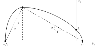
The plasticity part is based on the effective stresses and uses only a subset of the strains and stresses which are the normal stress \(\sigma_{\rm n}\) and the two shear stresses \(\sigma_{\rm s}\) and \(\sigma_{\rm t}\). The yield surface is composed of two ellipse which are arranged so that the transition of the two ellipses is smooth (Figure plastdamyieldfig).
Fig. 16 Latticeplastdam yield surface, which is composed of ellipse with a smooth transition.
Here parameters \(\alpha\) and \(\beta\) are the slopes, and \(f_{\rm c}\) and \(f_{\rm t}\) are the strength parameters shown in Figure plastdamyieldfig. The hardening function \(q\) controls the shape of the yield function.
[talpha] Thermal expansion coefficient. Default is 0.
[calpha] thermal displacement expansion coefficient. Optional parameter. Default
is 0.
e modulus of the equivalent lattice material
[a1] ratio of shear and normal modulus. Default is 1.
[a2] ratio of rotational and normal modulus. Default is 1.
fc compressive strength
angle1 friction angle
[ef] ductility of the hardening/softening function, default -1 (inactive); must
be > 0 when qres != 1; larger ef is more gradual (ef -> infinity is perfect plastic)
[angle2] cap aspect angle, default = angle1; angle2 < angle1 widens/raises the
compressive cap (maximum bond -> fc as angle2 -> 0)
[flowangle] dilatancy (flow) angle, default = angle1 (associated); set to 0 for
non-dilatant Coulomb contact
[qres] residual/asymptotic level of the hardening function, default 1 (perfect
plasticity); qres < 1 softens, qres > 1 hardens
[efp] exponent of the hardening function, default 1 (exponential); 2 gives a
Gaussian (zero slope at the peak)
This model combines a viscoelastic model, described in previous sections, with a linear elastic lattice material. Two material entries are used. One is for the viscoelastic lattice model and the other is for the viscoelastic model of choice.
The model description and parameters are summarized in Table 77.
Table 77 Visco elastic material model for lattice elements – summary.
This model combines a viscoelastic model, described in previous sections, with a damage lattice material model. Two material entries are used. One is for the viscoelastic extension of the damage lattice model and the other is for the viscoelastic model of choice.
The model description and parameters are summarized in Table 78.
Table 78 Damage visco elastic material model for lattice elements – summary.
[type] slip-law type: 0 = elastic-perfectly plastic; 1 = CEB bond-slip law
ascending branch then a constant plateau; 2 = full CEB bond-slip law (with the
descending/residual branch)
[s1], [s2], [s3], [alpha], [tf]
bond-slip law parameters with the same meaning as in the bondceb (CEB-FIP) model;
needed for type 1 and 2
This model combines a viscoelastic model, described in previous sections, with a plasticity damage lattice material model. Two material entries are used. One is for the viscoelastic extension of the plasticity damage lattice model and the other is for the viscoelastic model of choice.
The model description and parameters are summarized in Table 80.
Table 80 Plasticity-damage viscoelastic material model for lattice elements – summary
Elastic material model for lattice based frame elements
This is an elastic material model used together with lattice frame elements. It has been specifically developed to describe the failure of steel frame members using the lattice elements lattice3d and lattice3dnl. However, it can also be used with any other 3D lattice element, and with lattice2d in 2D (see below).
The stress-strain law has the form
\[\mathbf{s} = \mathbf{D}_{\rm e} \mathbf{e}\]
where \(\mathbf{e}\) is a vector of internal forces and moments, \(\mathbf{D}_{\rm e}\) is the elastic stiffness matrix, and \(\mathbf{e}\) is a vector of generalized strains obtained from displacement jumps smeared over the element length and rotational components. The model parameters are summarized in Table Table 82.
Table 81 Elastic model for 3D lattice based frame elements – summary.
Description
Elastic lattice model for frame elements
Record Format
latticeframeelasticind (rn)
[talpha (rn)] e (rn)n (rn)
[tcrit (rn)]
Parameters
material number
d material density
[talpha] Thermal expansion coefficient. Default is 0.
[tcrit] critical temperature \(T_{\rm crit}\) for the temperature dependent
reduction of the Young’s modulus (see below). Default is 0, which switches the reduction
off.
e Young’s modulus of the lattice material.
n Poisson’s ratio of the material that the beam element is made of.
The linear-elastic response of the frame elements is given directly as a relationship between generalized stress (internal forces) and generalized strain.
In 2D (lattice2d) the generalized strains and stresses reduce to the axial, shear and bending components, \(\mathbf{s} = (N, V, M_z)^T\), and the elastic stiffness is \(\mathbf{D}_{\rm e} = \mathrm{diag}(EA, G A_{\rm s}, E I)\), with the section properties provided by the element.
If tcrit is non-zero, the Young’s modulus (and thereby the shear modulus) is multiplied by the reduction factor
\[r(T) = \exp\left[ -\left( \dfrac{T - T_{\rm ref}}{T_{\rm crit} - T_{\rm ref}} \right)^2 \right] \qquad \textrm{for } T > T_{\rm ref} \textrm{ and } T > 0\]
and \(r = 1\) otherwise. Here \(T\) is the temperature at the integration point, the sum of the element temperature loads and of a registered temperature field (e.g. from a staggered thermo-mechanical analysis), and \(T_{\rm ref}\) is the reference temperature (referencetemperature of the structural material, default 0).
Steel Plasticity material model for lattice based frame elements
This is a plasticity material used together with lattice frame elements. It has been specifically developed to describe the failure process of steel frame members using the lattice elements lattice3d and lattice3dnl. It can also be used with lattice2d, for example to model yielding reinforcement bars in 2D.
where \(\mathbf{e}\) is a vector of internal forces and moments, \(\mathbf{D}_{\rm e}\) is the elastic stiffness matrix, \(\mathbf{e}\) is a vector of generalised strains obtained from displacement jumps smeared over the element length and rotational components, and \(\mathbf{e}_{\rm p}\) are the plastic strains. The model parameters are summarised in Table Table 82.
Table 82 Plasticity steel model for 3D lattice frame elements – summary
[talpha] Thermal expansion coefficient. Default is 0.
[tcrit] critical temperature \(T_{\rm crit}\) for the temperature dependent
reduction of the Young’s modulus and of the capacities by the factor \(r(T)\) given
for latticeframeelastic. Default is 0, which switches the reduction off.
e Young’s modulus of the lattice material.
n Poisson’s ratio of the material that the beam element is made of.
[sigmay] yield stress. If given, the capacities are computed from the cross
section: for a circle of radius \(r\), \(N_0=\sigma_y \pi r^2\),
\(M_{y0}=M_{z0}=4\sigma_y r^3/3\) and \(M_{x0}=\sigma_y J/r\); for a rectangle
\(b_y \times b_z\), \(N_0=\sigma_y b_y b_z\), \(M_{y0}=\sigma_y b_y b_z^2/4\)
and \(M_{z0}=\sigma_y b_z b_y^2/4\). Otherwise nx0, mx0,
my0 and mz0 are required.
[nx0] ultimate capacity under pure axial loads.
[mx0] ultimate capacity under pure moment about \(x\).
[my0] ultimate capacity under pure moment about \(y\).
[mz0] ultimate capacity under pure moment about \(z\).
[sub] maximum number of subincrementations. Default is 10.
[iter] maximum number of newton iterations. Default is 100.
[tol] tolerance for newton method. Default is \(10^{-6}\).
[htype] type of hardening law. 0: linear, \(h(\kappa) = 1 + H\kappa\);
1: piecewise linear, given by h_eps and h(eps). Default is 0.
[h] hardening modulus \(H\) of the linear law (htype0). Default is 0
(perfect plasticity).
[h_eps] values of the hardening variable \(\kappa\) for the piecewise linear
law (htype1). The first entry must be 0, and \(\kappa\) must not exceed the last
entry.
[h(eps)] values of the hardening function \(h\) at the points
h_eps; same size as h_eps. The first entry is normally 1.
[hlength] length \(l_{\rm h}\) that converts the rotational plastic strains
into the hardening variable \(\kappa\) (see below). Default is 0, for which only the
axial plastic strain drives hardening.
[capmode] 0: nx0, mx0, my0 and mz0 are
resultants; 1: they are given per unit width and multiplied by the tributary width of
the element (the shell width of lattice3d shells, 1 otherwise). Default is 0.
The nonlinear response of the beam element is given directly as a relationship between internal force and strain. The basic equations include an additive decomposition of total strain into elastic part and plastic part of the form
where \(N_x\), \(M_x\), \(M_y\) and \(M\), are the two components of bending moment, an axial force and a torsional moment, respectively. The corresponding components with the subscript 0 indicate a fully plastic value under the condition that each component of resultant forces acts independently.
with \(h(\kappa) = 1 + H\kappa\) for htype0 and the piecewise linear function defined by h_eps and h(eps) for htype1. The hardening variable evolves as
where \(\dot{e}_{{\rm p}N}\) is the axial plastic strain rate and \(\dot{e}_{{\rm p}M_x}\), \(\dot{e}_{{\rm p}M_y}\) and \(\dot{e}_{{\rm p}M_z}\) are the plastic rates of twist and curvature. The length \(l_{\rm h}\) (hlength) converts these rotational components into strains. With the default \(l_{\rm h} = 0\), plastic bending does not cause hardening, so hlength must be set for members that harden in bending.
Reinforced concrete plasticity-damage material model for lattice based frame elements
This is a plasticity-damage material used together with 3d lattice frame elements. It has been specifically developed to describe the failure process of reinforced concrete frame members using the lattice elements lattice3d and lattice3dnl.
where \(\mathbf{e}\) is a vector of internal forces and moments, \(\mathbf{D}_{\rm e}\) is the elastic stiffness matrix, \(\mathbf{e}\) is a vector of translation and rotational jumps smeared over the element length and \(\mathbf{e}_{\rm p}\) are the plastic smeared jumps. The model parameters are summarised in Table Table 82.
Table 83 Damage Plasticity concrete model for 3D lattice frame elements – summary
Description
Damage-plasticity lattice model for reinforced concrete
[talpha] Thermal expansion coefficient. Default is 0.
[tcrit] critical temperature \(T_{\rm crit}\) for the temperature dependent
reduction of the capacities by the factor \(r(T)\) given for latticeframeelastic; the
elastic stiffness is not reduced. Default is 0, which switches the reduction off.
e Young’s modulus of the lattice material.
n Poisson’s ratio of the material that the beam element is made of.
nx0 ultimate positive capacity under pure axialloads.
mx0 ultimate positive capacity under pure moment about \(x\).
my0 ultimate positive capacity under pure moment about \(y\).
mz0 ultimate positive capacity under pure moment about \(z\).
nx1 ultimate negative capacity under pure axialloads.
mx1 ultimate negative capacity under pure moment about \(x\).
my1 ultimate negative capacity under pure moment about \(y\).
mz1 ultimate negative capacity under pure moment about \(z\).