Nonlinear isotropic material for moisture transport - NlIsoMoisture

Nonlinear isotropic material for moisture transport – NlIsoMoisture

This is a more general model for nonlinear moisture transport in isotropic porous materials, based on a nonlinear sorption isotherm (relation between the pore relative humidity \(h\) and the water content \(w\)) and on a humidity-dependent moisture permeability. The governing differential equation solves water mass balance in a unit volume [kg/m³/s] and reads

(121)\[k(h) \frac{\partial h}{\partial t} = \nabla \cdot \left[ c(h) \nabla h \right] + w_n \frac{\partial \alpha}{\partial t}\]

where \(k(h)\) [kg/m³] is the humidity-dependent moisture capacity (\(k(h)=\frac{\partial w}{\partial h}\) which is derivative of the moisture content \(w(h)\) [kg/m³] with respect to the relative humidity), \(c(h)\) [kg/m/s] is the moisture permeability and the sink term \(w_n \frac{\partial \alpha}{\partial t}\) corresponds to non-evaporable water loss due to hydration. \(w_n\) is non-evaporable water content for complete hydration per m³ [kg/m³] and \(\alpha\) is degree of hydration [-]. For the majority of cements, 1 kg of cement consumes approximately 0.23 kg of non-evaporable water at complete hydration.

So far, six different functions for the sorption isotherm have been implemented (in fact, what matters for the model is not the isotherm itself but its derivative—the moisture capacity):

Isotherms

• Isotherm proposed by Kuenzel [Kuenzel] (isothermType=3) in the form

(122)\[w(h) = w_f \frac{(b-1)h}{b-h}\]

where \(w_f\) [kg/m³] is the moisture content at free saturation and \(b\) is a dimensionless approximation factor greater than 1.

• Isotherm proposed by Hansen [Hansen] (isothermType=4) in the form

(123)\[u(h) = u_h \left(1- \frac{\ln h}{A} \right)^{-1/n}\]

characterizes the amount of adsorbed water by the moisture ratio \(u\) [kg/kg]. To obtain the moisture content \(w\), it is necessary to multiply the moisture ratio by the density of the solid phase. In ((123)), \(u_h\) is the maximum hygroscopically bound water by adsorption, and \(A\) and \(n\) are constants obtained by fitting of experimental data.

• The BSB isotherm [BSB] (isothermType=5) is an improved version of the famous BET isotherm. It is expressed in terms of the moisture ratio

(124)\[u(h) = \frac{C k V_m h}{(1-k h)(1+(C-1)k h)}\]

where \(V_m\) is the monolayer capacity, and \(C\) depends on the absolute temperature \(T\) and on the difference between the heat of adsorption and condensation. Empirical formulae for estimation of the parameters can be found in [Xi]. Note that these formulae hold quite accurately for cement paste only; a reduction of the moisture ratio is necessary if the isotherm should be applied for concrete.

• Bilinear isotherm (isothermType=6) is defined by its moisture capacity capa for relative humidity less than hx. Parameter wf defines moisture content at full saturation, \(h = 1\). Convergence is substantially improved by a smooth transition on interval \((hx-dx, hx+dx)\). Similarly to the linear isotherm the moisture content can be adjusted by parameter isooffset.

The present implementation covers three functions for moisture permeability:

Moisture Permeability

• Piecewise linear permeability (permeabilityType=0) is defined by two arrays with the values of pore relative humidity \(perm\_h\) and the corresponding values of moisture content \(perm\_c(h)\). The arrays must be of the same size.

The Bažant-Najjar permeability function (\(permeabilityType=1\)) is given by the same formula ((120)) as the diffusivity in Section Isotropic material for moisture transport based on Bažant and Najjar – BazantNajjarMoisture. All parameters have a similar meaning as in ((120)) but \(c1\) is now the moisture permeability at full saturation [kg/m\(\cdot\)s].

The permeability function proposed by Xi et al. [Xi] (\(permeabilityType=2\)) reads

(125)\[c(h) = \alpha_h + \beta_h \left[ 1 - 2^{-10^{\gamma_h(h-1)}} \right]\]

where \(\alpha_h\), \(\beta_h\) and \(\gamma_h\) are parameters that can be evaluated using empirical mixture-based formulae presented in [Xi]. However, if those formulae are used outside the range of water-cement ratios for which they were calibrated, the permeability may become negative. Also the physical units are unclear.

Note that the Bajant-Najjar model from Section Isotropic material for moisture transport based on Bažant and Najjar – BazantNajjarMoisture can be obtained as a special case of the present model if \(permeabilityType\) is set to 1 and \(isothermType\) is set to 0. The ratio \(c1/moistureCapacity\) then corresponds to the diffusivity parameter \(C_1\) from (119).

The model parameters are summarized in Table 63.

Table 63 Nonlinear isotropic material for moisture transport

Description	Nonlinear isotropic material for moisture transport
Record Format	NlIsoMoistureMat num (in) d (rn) isothermType (in) permeabilityType (in) [rhodry (rn)] [capa (rn)] [iso_h (ra)] [iso_w(h) (ra)] [dd (rn)] [wf (rn)] [b (rn)] [uh (rn)] [A (rn)] [nn (rn)] [c (rn)] [k (rn)] [Vm (rn)] [hx (rn)] [dx (rn)] [perm_h (ra)] [perm_c(h) (ra)] [c1 (rn)] [n (rn)] [alpha0 (rn)] [hc (rn)] [alphah (rn)] [betah (rn)] [gammah (rn)] [wn (rn)] [alpha (expr)]
Parameters	num material model number d material density isothermType isotherm function as listed above (0, 1, …6) permeabilityType moisture permeability function as listed above (0, 1, 2) rhodry [kg/m\(^3\)] density of dry material (for \(isothermType=4\) and 5) capa [kg/m\(^3\)] moisture capacity (for \(isothermType=0\) and 6) isooffset [kg/m\(^3\)] moisture capacity at zero relative humidity (for \(isothermType=0\) and 6) iso_h [-] humidity array (for \(isothermType=1\)) iso_w(h) [kg/m\(^3\)] moisture content array (for \(isothermType=1\)) dd [-] parameter (for \(isothermType=2\)) wf [kg/m\(^3\)] is the moisture content at free saturation (for \(isothermType=3\) and 6) b [-] parameter (for \(isothermType=3\)) uh [kg/kg] maximum hygroscopically bound water by adsorption (for \(isothermType=4\)) A [-] parameter (for \(isothermType=4\)) n [-] parameter (for \(isothermType=4\)) Vm (for \(isothermType=5\)) k (for \(isothermType=5\)) C (for \(isothermType=5\)) hx [-] transition relative humidity (for \(isothermType=6\)) dx [-] length of the smooth transition (for \(isothermType=6\)) perm_c(h) [kg m\(^{-1}\) s\(^{-1}\)] moisture permeability array (for \(permeabilityType=0\)) c1 [kg m\(^{-1}\) s\(^{-1}\)] moisture permeability at full saturation (for \(permeabilityType=1\)) n [-] exponent (for \(permeabilityType=1\)) alpha0 [-] ratio between minimum and maximum diffusivity (for \(permeabilityType=1\)) hc [-] relative humidity at which the diffusivity is exactly between its minimum and maximum value (for \(permeabilityType=1\)) alphah [kg m\(^{-1}\) s\(^{-1}\)] (for \(permeabilityType=2\)) betah [kg m\(^{-1}\) s\(^{-1}\)] (for \(permeabilityType=2\)) gammah [-] (for \(permeabilityType=2\)) wn [kg m\(^{-3}\)] nonevaporable water content per m\(^3\) of concrete, default 0.23 kg/kg of cement alpha [-] function of degree of hydration
Supported modes	_2dHeat
Tests/Examples	tm/nlisomoisture01.in, tm/nlisomoisture02.in, tm/nlisomoisture03.in

CemhydMat

CemhydMat represents a hydrating material based on CEMHYD3D model version 3.0, developed at NIST [NISTIR7232]. The model represents a digital hydrating microstructure, driven with cellular automata rules and combined with cement chemistry. Ordinary Portland cement is treated without any difficulties, blended cements are usually decomposed into hydrating Portland contribution and intert secondary cementitious material. The microstructure size can be from \(10\times10\times10\) to over \(200\times200\times200\) \(\mu\text{m}\). For standard computations the size \(50\times50\times50\) suffices.

Each material instance creates an independent microstructure. It is also possible to enforce having different microstructures in each integration point. The hydrating model is coupled with temperature and averaging over shared elements within one material instance occurs during the solution. Such approach allows domain partitioning to many CemhydMat instances, depending on expected accuracy or computational speed. A more detailed description with engineering examples was published [Smilauer:09]. Table 64 summarizes input parameters.

Table 64 Cemhydmat - summary

Description	Cemhyd - hydrating material
Record Format	CemhydMat num (in) d (rn) k (rn) c (rn) file (s) [eachGP (in)] [densityType (in)] [conductivityType (in)] [capacityType (in)] [castingtime (rn)] [nowarnings (ia)] [scaling (ra)] [reinforcementDegree (rn)]
Parameters	num material model number d material density k Conductivity c Specific heat capacity file XML input file for cement microstructure and concrete composition eachGP 0 (default) no separate microstructures in each GP, 1 assign separate microstructures to each GP densityType 0 (default) get density from OOFEM input file, 1 get it from XML input file conductivityType 0 (default) get constant conductivity from OOFEM input file, 1 compute as \(\lambda = \textrm{k} (1.33-0.33\alpha)\) [Ruiz:01] capacityType 0 (default) get capacity, 1 according to Bentz, 2 according to XML and CEMHYD3D routines castingtime optional casting time of concrete, from which hydration takes place. Absolute time is used. nowarnings supresses warnings when material data are out of standard ranges. The array of size 4 represent entries for density, conductivity, capacity, temperature. Nonzero values mean supression. scaling components in the array scale density, conductivity, capacity in this order. nowarnings are checked before scaling. reinforcementDegree specifies the area fraction of reinforcement. Typical values is 0.015. Steel reinforcement slightly increases concrete conductivity and slightly decreases its capacity. Thermal properties of steel are considered 20 W/m/K and 500 J/kg/K.
Supported modes	_2dHeat, _3dHeat
Tests/Examples	tmcemhyd/cemhyd01.in, tmcemhyd/cemhyd02.in

The input XML file specifies the details about cement and concrete composition. It is possible to start all simulations from the scratch, i.e. with the reconstruction of digital microstructure. Alternatively, the digital microstructure can be provided directly in two files; one for chemical phases, the second for particle’s IDs. The XML input file can be created with the CemPy package, obtainable from http://mech.fsv.cvut.cz/~smilauer/index.php?id=software. The CemPy package alleviates tedious preparation of particle size distribution etc.

The linear solver (specified as NonStationaryProblem) performs well when the time integration step is small enough (order of minutes) and heat capacity, conductivity and density remain constant. If not so, use of nonlinear solver is strongly suggested (specified as NlTransientTransportProblem).

HydratingConcreteMat

Simple hydration models based on chemical affinity are implemented. The models calculate the degree of hydration of cement, \(\alpha\), which can be scaled to the level of concrete when providing the corresponding amount of cement in concrete. Blended cements can be considered as well, either by separating supplementary cementitious materials from pure Portland clinker or by providing parameters for the evolution of hydration degree and potential heat. The released heat from the cement paste is obtained from

\[Q(t) = \alpha Q_{pot},\]

where the potential hydration heat, \(Q_{pot}\), is expressed in kJ/kg of cement and for pure Portland cement is around 500 kJ/kg.

Evolution of hydration degree under isothermal curing conditions is approximated by several models. Scaling from a reference temperature to arbitrary temperature is based on the Arrhenius equation, which coincides with the maturity method approach. The equivalent time, \(t_e\), is defined as the time under constant reference (isothermal) temperature

\[\begin{split}t_e(T_0) &= t(T) k_{rate},\\ k_{rate} &= \exp\left[\frac{E_a}{R}\left(\frac{1}{T_0} - \frac{1}{T}\right)\right],\end{split}\]

where \(t\) is real time, \(T\) is the arbitrary constant temperature of hydration, \(T_0\) is a reference temperature, \(R\) is the universal gas constant (8.314 Jmol\(^{-1}\)K\(^{-1}\)), and \(E_a\) is the apparent activation energy. Due to the varying history of temperature, an incremental solution is adopted. Linear and nonlinear nonstationary solvers are supported for all hydrationmodeltype’s. Hydration models are evaluated at intrinsic time in each time step. Usually, intrinsic time is in the middle of the time step.

The hydrationmodeltype = 1 is based on an exponential approximation of hydration degree [Schindler:2005]. An equivalent time increment is added in each time step. Thus, all the thermal history is stored in the equivalent time

\[\alpha(t_e) = \alpha_\infty \exp\left(-\left[\frac{\tau}{t_e}\right]^\beta\right)\]

where three parameters \(\tau\), \(\beta\), and \(\alpha_\infty\) are needed. Some meaningful parameters are provided in [Schindler:2005], e.g., \(\tau=26\cdot3600=93600\) s, \(\beta=0.75\), and \(\alpha_\infty=0.90\).

The hydrationmodeltype = 2 is inspired by Cervera et al. [Cervera:99], who proposed an analytical form of the normalized affinity which was refined in [Gawin:06a]. A slightly modified formulation is proposed here. The affinity model is formulated for a reference temperature 25°C

(126)\[\begin{split}\frac{\partial \alpha}{\partial t} &=& \tilde{A}_{25}(\alpha) k_{rate}= B_1 \left( \frac{B_2}{\alpha_\infty} + \alpha \right ) \left( \alpha_\infty - \alpha \right) f_s \exp\left(-\bar{\eta}\frac{\alpha}{\alpha_\infty}\right) k_{rate}\\ \alpha &>& DoH_1 \Rightarrow f_s = 1+P_1(\alpha - DoH_1)~\mathrm{else}~f_s = 1\end{split}\]

where \(B_1, B_2\) are coefficients to be calibrated, \(\alpha_\infty\) is the ultimate hydration degree and \(\bar{\eta}\) represents microdiffusion of free water through formed hydrates. The function \(f_s\) adds additional peak which may occur in slag-rich blended cements with two parameters \(DoH_1,P_1\). The solution proceeds incrementally, where \(\alpha\) is the unknown. During one macroscopic time step, (126) needs to be integrated in finer inner steps. This is controlled with two optional variables; maxmodelintegrationtime specifies maximum integration time in the loop while minmodeltimestepintegrations specifies minimum number of integration steps.

Table 65 HydratingConcreteMat - summary of affinity hydration models.

Description	HydratingConcreteMat
Record Format	HydratingConcreteMat num (in) d (rn) k (rn) c (rn) hydrationmodeltype (in) Qpot (rn) masscement (rn) [activationenergy (rn)] reinforcementdegree (rn)] [densitytype (in)] [conductivitytype (in)] [capacityType (in)] [minModelTimeStepIntegrations (in)] [maxmodelintegrationtime (rn)] [castingTime (rn)]
Parameters	num material model number d material density about 2300 kg/m\(^3\) k Conductivity about 1.7 W/m/K c Specific heat capacity about 870 J/kg/K hydrationmodeltype 1 is exponential model from refeqeq:affinity1, 2 is affinity model from refeqeq:affinity2 Qpot Potential heat of hydration, about 500 kJ/kg of cement masscement Cement mass per 1m\(^3\) of concrete, about 200-450 activationenergy Arrhenius activation energy, 38400. (default) DoHinf degree of hydration at infinite time B1,B2,eta,DoH1,P1 parameters from refeqeq:affinity2-refeqeq:affinity3 reinforcementDegree specifies the area fraction of reinforcement. Typical values is 0.015. Steel reinforcement slightly increases concrete conductivity and slightly decreases its capacity. Thermal properties of steel are considered 20 W/m/K and 500 J/kg/K. densityType 0 (default) conductivityType 0 (default), 1 compute as \(\lambda = \textrm{k} (1.33-0.33\alpha)\) [Ruiz:01] capacityType 0 (default) minModelTimeStepIntegrations Minimum integrations per time step in affinity model 30 (default) maxmodelintegrationtime Maximum integration time step in affinity model 36000 s (default) castingtime optional casting time of concrete, from which hydration takes place, in s relmatage material age at casting time, 0 s (default) scaling components in the array scale density, conductivity, capacity in this order. nowarnings are checked before scaling.
Supported modes	_2dHeat, _3dHeat
Tests/Examples	tm/TwoStepCasting_01.in, tm/hydratingConcreteMat01.in, tm/hydratingConcreteMat02.in, tm/hydratingConcreteMat03.in, tm/hydratingConcreteMat04.in, tm/hydratingConcreteMat05.in, tm/hydratingConcreteMat06.in, tm/hydratingConcreteMat07.in

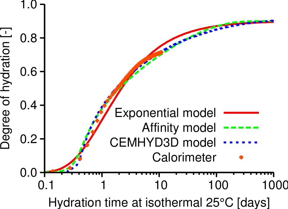
Fig. 15 Performance of implemented hydration models: exponential model from eq:affinity1, affinity model from (126), CEMHYD3D model from Subsection CemhydMat.

Parameters for exponential model according to eq:affinity1 are \(\tau=26\cdot3600=93600\) s, \(\beta=0.75\), \(\alpha_\infty=0.90\). Parameters for affinity model according to (126) are \(B_1=3.519e-4\) s^-1, \(B_2=8.0e-7\), \(\eta=7.4\), \(\alpha_\infty=0.85\).