Grassl Group
Concrete Mechanics for Performance Based Design
LS-DYNA examples for using CDPM2 (Student projects)
Below are example LS-DYNA analyses using CDPM2 (Concrete Damage–Plasticity Model 2) for MSc and undergraduate projects. For general setup guidance, see the Info for student projects.
Quick start
Download the ready-to-use package (mesh template, material/control examples, simple Perl tools):
- Generate mesh with T3D
- Convert T3D mesh to LS-DYNA keywords
- Run LS-DYNA (example: 8 cores)
t3d -d 0.02 -p 8 -i mesh.in -o mesh.out
perl t3d2lsdyna.pl mesh.out > mesh.k
lsdyna i=input.k ncpu=8 > std.out &
Visualise: open d3plot in LS-PrePost. For curves, use the included Perl scripts (e.g., reaction.pl).
Outline
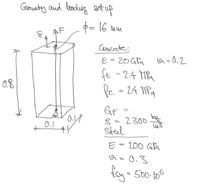
Example: Reinforced concrete prism subjected to tension (LS-DYNA)
We demonstrate the LS-DYNA pipeline on a prism with a single central rebar tensioned through the bar.
Discrete reinforcement is modelled with beam/truss elements. Typical options:
- (a) rebar constrained in the solid mesh,
- (b) shared nodes between rebar and solid,
- (c) coincident nodes with slip (see DOI; inputs linked from LS-DYNA page).
Pipeline
- Generate mesh with T3D
- Convert T3D output to LS-DYNA format
- Create control and material files; adjust
mesh.kin LS-PrePost - Run LS-DYNA
- Postprocess with LS-PrePost and Perl scripts
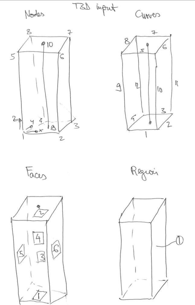
1) Generate mesh with T3D
We use T3D because it creates robust tetra meshes and supports rebar options. Constant-strain tets are suitable for localisation in nonlinear fracture analyses.
Typical command:
t3d -d 0.02 -p 8 -i mesh.in -o mesh.out
Central rebar (curve 13) written to output (option a/b)
curve 13 order 2 vertex 9 10 output yes
Faces (patches)
# bottom / top / front / back / left / right
patch 1 normal 0 0 1 boundary curve 1 2 3 4
patch 2 normal 0 0 1 boundary curve 5 6 7 8
patch 3 normal 0 -1 0 boundary curve 1 10 -5 -9
patch 4 normal 0 -1 0 boundary curve -3 11 7 -12
patch 5 normal 1 0 0 boundary curve -4 12 8 -9
patch 6 normal 1 0 0 boundary curve 2 11 -6 -10
Region
region 1 boundary patch -1 2 3 -4 -5 6 size def
For shared nodes (option b), “fix” the rebar vertices in the faces and region:
# patches containing control vertices
patch 1 normal 0 0 1 boundary curve 1 2 3 4 fixed vertex 9
patch 2 normal 0 0 1 boundary curve 5 6 7 8 fixed vertex 10

# region includes rebar curve as fixed
region 1 boundary patch -1 2 3 -4 -5 6 size def fixed curve 13
Interactive meshing (if T3D built with X11):
t3d -X -d 0.02 -p 8 -i mesh.in -o mesh.out
2) Convert to LS-DYNA format
Minimal converter usage:
perl t3d2lsdyna.pl mesh.out > mesh.k
The script reads node/element blocks from mesh.out and writes LS-DYNA *NODE/*ELEMENT blocks to mesh.k.
3) Control & material files; LS-PrePost adjustments
Keep three files per model:
input.k— analysis controls, includes, BCs, loadsmaterial.k— material cards (concrete & steel)mesh.k— nodes/elements/sets (edit this one with LS-PrePost only)
In LS-PrePost, create node sets (e.g., the nodes at vertices 9 and 10) and a beam set for the rebar. See your internal tutorial for creating sets.
CDPM2 material via user model (abridged):
*MAT_USER_DEFINED_MATERIAL_MODELS
$#     mid        ro        mt       lmc       nhv    iortho     ibulk        ig
         1    2.30E3        50        26        27         0        25        26
$#   ivect     ifail    itherm    ihyper      ieos      lmca
         1         0         0         0         0         0
$    p1(E)    p2(PR)      ...                 p5(FT)   p6(FC)   p7(HP)
  20.e9       0.2                              2.4e6    24.e6     0.01
$  p17(WF)  ...                      p22(EFC)
 103.7e-6                             1.0e-3
Steel (rebar) — bilinear plasticity:
*MAT_PLASTIC_KINEMATIC
$#     mid        ro         e        pr      sigy      etan      beta
         2    7.85E3    200.E9       0.3    500.E6        0.       0.0
Parts and sections:
*PART
solid
$#      pid     secid       mid
         1         1         1
*PART
reinforcement
$#      pid     secid       mid
         2         2         2

*SECTION_SOLID
$    secid    elform
         1        10    $ constant-strain tets

*SECTION_BEAM_TITLE
Section reinforcement
$    secid    elform      shrf   qr/irid   cst
         2         1       1.0         2     1
Embed discrete rebar into solid (option a):
*CONSTRAINED_BEAM_IN_SOLID
$    slave    master     sstyp     mstyp
         2         1         1         1
Includes:
*INCLUDE
material.k
*INCLUDE
mesh.k
BCs and prescribed displacement:
*BOUNDARY_SPC_SET
$ ID   CID  DOFX DOFY DOFZ DOFRX DOFRY DOFRZ
  1     0     1    1    1     0     0     0   $ fix bottom rebar node (v=9)

*BOUNDARY_SPC_SET
$ ID   CID  DOFX DOFY DOFZ DOFRX DOFRY DOFRZ
  2     0     1    1    0     0     0     0   $ fix x,y at top rebar node (v=10)

*BOUNDARY_PRESCRIBED_MOTION_SET
$  ID  DOF  VAD  LCID   SF
   1    3    2   111   1.0    $ z-displacement at top node set

*DEFINE_CURVE
111, 0, 1., 1., 0., 0.
 0.0,     0.0
 &Tend,   &MaxDisp
 &Tend2,  &MaxDisp
Output:
*DATABASE_NODFOR
 &TASCII
*DATABASE_SPCFORC
 &TASCII
*DATABASE_BINARY_D3PLOT
 &TDplot
*DATABASE_EXTENT_BINARY
$ neiph ... sigflg epsflg ...
         5               1      1
4) Run LS-DYNA
Use screen so jobs continue after disconnect:
screen
Then launch (example with 8 cores):
lsdyna i=input.k ncpu=8 > std.out &
Use a modest core count to share cluster resources. Reduce runtime by coarser meshes and/or faster loading, but avoid excessive dynamics.
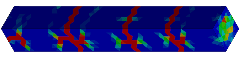
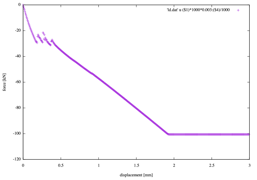
5) Postprocess results
In LS-PrePost, plot maximum principal strain (apply an upper threshold) to visualise cracks. Extract curves with Perl tools:
perl reaction.pl spcforc > output.dat
Single-element example (LS-DYNA)
Coming soon.
Last updated by Peter Grassl