Coupling flow and mechanics on a lattice — a fluid-pressurised thick-walled cylinder

The mechanical lattice deforms; the transport lattice carries flow. This post couples them: a fluid pressure inside a thick-walled cylinder drives the wall outward through Biot's effective stress — and the lattice reproduces the closed-form poroelastic solution, including the way Biot's coefficient flips the wall from thinning to thickening.

The fracture posts on this site use the mechanical lattice — frame elements along the Delaunay edges of a random point set, deforming under load. The flow series introduced the transport lattice — conduit elements along the dual Voronoi edges, carrying pore fluid. They share the same Voronoi–Delaunay mesh but live on opposite sides of the duality.

This post couples the two. Pore pressure computed on the transport lattice acts on the mechanical lattice through Biot’s effective stress, and the mechanical response feeds back. It reproduces the elastic part of the thick-walled-cylinder benchmark from Grassl, Fahy, Gallipoli & Wheeler (2015), A hydro-mechanical lattice approach for modelling hydraulic fracture (J. Mech. Phys. Solids 75, 104–118) — the precursor to fluid-driven fracture.

The problem

A saturated thick-walled cylinder (annulus): inner radius r_i, outer radius r_o. A fluid pressure is prescribed on the inner cavity wall and the outer surface is drained (zero pressure). With negligible storage the transport problem reaches steady state, so the pore pressure follows the classic logarithmic radial profile

P_f(r) = P_fi · ln(r_o / r) / ln(r_o / r_i),

high at the cavity, zero at the outer rim. That field is what loads the mechanics.

How the pressure loads the solid

Total stress is effective (mechanical) stress plus a fraction of the pore pressure:

σ = σ_eff + b · P_f,

where b is Biot’s coefficient. Two limits bracket the behaviour, and they are qualitatively opposite:

• b = 0. The pore pressure enters only as a traction on the cavity wall — a classic internally pressurised cylinder. The cavity expands far more than the outer rim, so the wall thins.
• b = 1 (full Biot). The pore pressure also acts as a distributed body force throughout the wall (its gradient pushes the solid outward everywhere). The whole wall moves out, the outer rim slightly more than the inner — so the wall thickens.

Biot’s coefficient flips the sign of the wall-thickness change. That is the headline result, and it is exactly what the analytical solution in the 2015 paper (Appendix A, eq. A.22) predicts.

Lattice vs analytical

The radial displacement u_r, normalised by r_i, against the normalised radius r / r_i, for both Biot coefficients — raw lattice nodes (scatter) against the closed-form solution (lines):

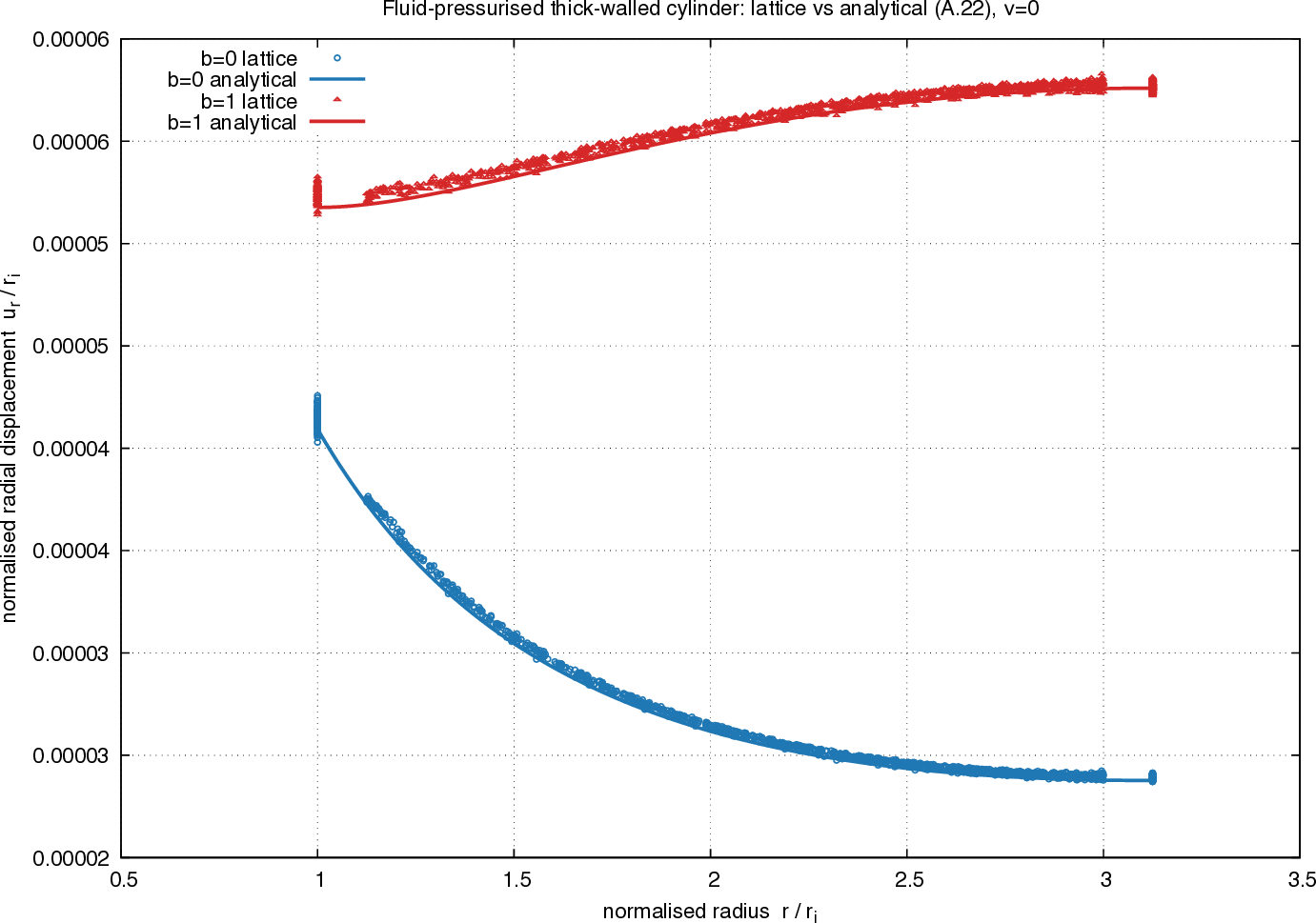
The two cases separate cleanly: b = 0 decreases with radius (thinning), b = 1 increases (thickening), and the lattice scatter sits on the analytical curves. The same contrast in space — the displacement magnitude u_r / r_i on the undeformed mesh, both panels on a common colour scale:

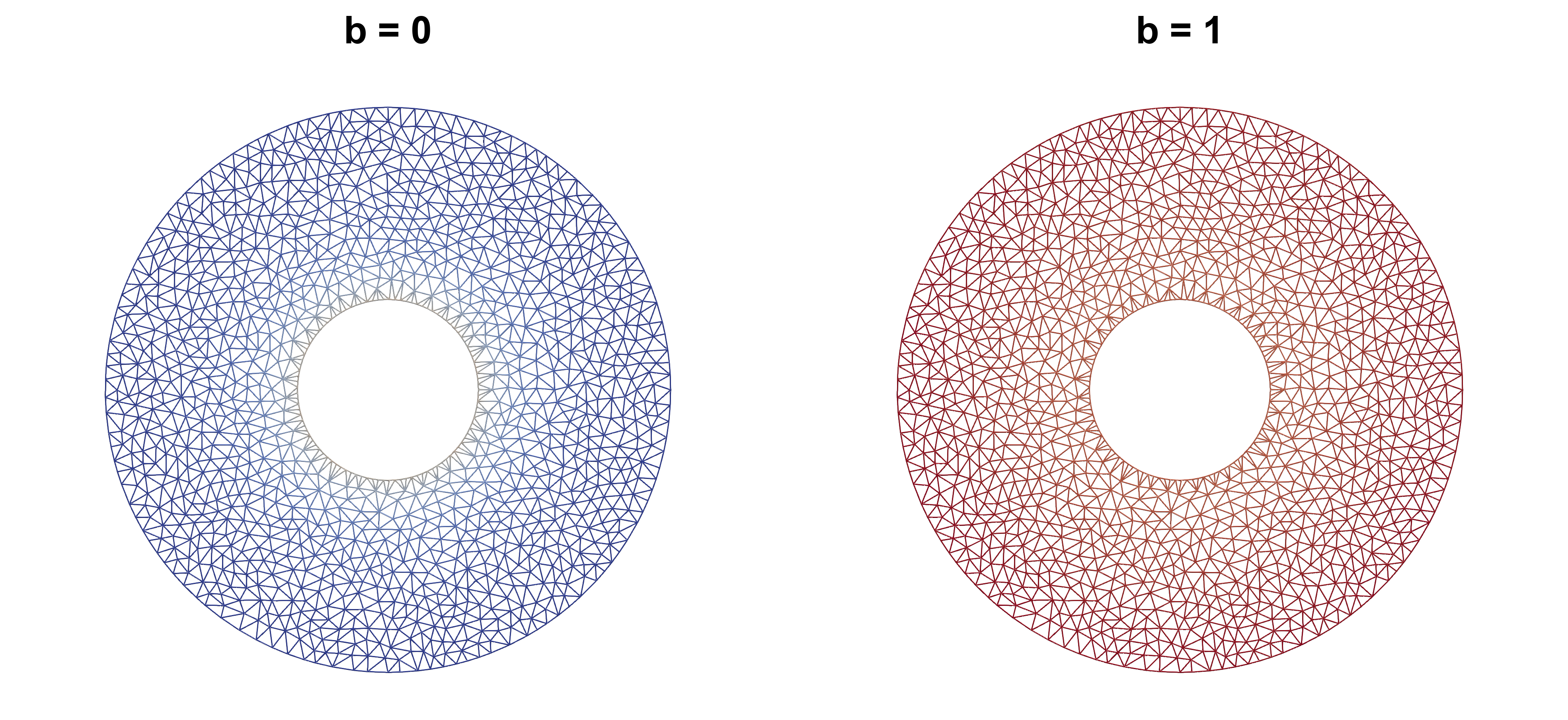
Blue is small displacement. Red is large displacement. b = 0 has more small displacement with a strong radial gradient (large at the cavity, small at the rim); b = 1 has far more large displacement and more uniform. Same pressure field, opposite wall response.

The ratios — inner vs outer, i.e. the thinning-versus-thickening signature that is the whole point — match closely. The angular scatter at a given radius comes from the mesh at the boundary.

This elastic, uncracked case is the baseline. The same coupled lattice — pore pressure on the Voronoi dual, effective stress on the Delaunay frame — can drive fracture: raise the cavity pressure until the wall cracks, the hydraulic-fracturing problem of the 2015 paper.

Reproduce

git clone https://github.com/githubgrasp/oofem-examples.git
cd oofem-examples/lattice-coupling-pressure-2d
docker run --rm -v "$PWD":/work ghcr.io/githubgrasp/oofem-public:lattice-coupling-pressure-2d bash run.sh

Each Biot case is a self-contained sub-folder (b0/, b1/) that can also be run on its own (bash b0/run.sh); the two differ only by the bio value in control.in. The full two-case run takes about half a minute.

The :lattice-coupling-pressure-2d image tag is immutable — use :latest instead to track the current OOFEM build (results may drift slightly as the code evolves).

Built with OOFEM.

← All posts