3D Continuum Elements

3D Continuum Elements

This section contains description of continuum elements.

LSpace element

Implementation of Linear 3d eight - node finite element. Each node has 3 degrees of freedom. The element features are summarized in Table 32.

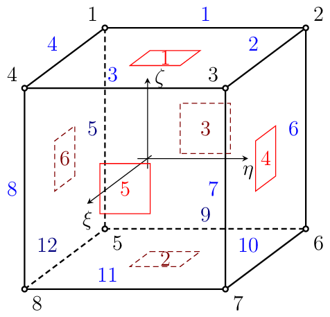
Fig. 12 LSpace element (Node numbers in black, side numbers in blue, and surface numbers in red).

Table 32 lspace element summary

Keyword	lspace
Description	Linear isoparametric brick element
Specific parameters	[NIP (in)]
Parameters	NIP: allows to set the number of integration points (possible completions are 1, 8 (default), or 27).
Unknowns	Three dofs (u-displacement, v-displacement, w-displacement) are required in each node.
Approximation	Linear approximation of displacement and geometry.
Integration	Full integration of all strain components.
Features	Supports adaptivity, geometric nonlinearity, and layered cross section support
CS properties
Loads
Nlgeo	0,1,2.
Status	Reliable
Tests/Examples	sm/python/usrdefboundaryload01.in, smmfront/mfront01.in, sm/deadweight02.in, sm/brick_nlgeo_1.in, sm/blatzko1.in, sm/brick_nlgeo_2.in, sm/brick_nlgeo_3.in, sm/brick_nlgeo_4.in, sm/brick_nlgeo_5.in, sm/brick_nlgeo_6.in (and 30 more)

LSpaceBB element

Implementation of 3d brick eight - node linear approximation element with selective integration of deviatoric and volumetric strain contributions (B-bar formulation) for incompressible problems. Features and description identical to conventional lspace element, see section LSpace element.

QSpace element

Implementation of quadratic 3d 20-node finite element. Each node has 3 degrees of freedom. The element features are summarized in Table 33.

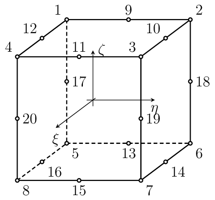
Fig. 13 QSpace element.

Table 33 qspace element summary

Keyword	qspace
Description	Quadratic isoparametric brick element
Specific parameters	[NIP (in)]
Parameters	NIP: allows to set the number of integration points (possible completions are 1, 8 (default), or 27).
Unknowns	Three dofs (u-displacement, v-displacement, w-displacement) are required in each node.
Approximation	Quadratic approximation of displacement and geometry.
Integration	Full integration of all strain components.
Features	Layered cross section support.
CS properties
Loads
Nlgeo	0,1,2.
Status	Reliable
Tests/Examples	sm/layered_cube_lcs.in, sm/layered_cube.in, sm/vitrification01.in, sm/cantilever_Qspace.in

LTRSpace element

Implementation of tetrahedra four-node finite element. Each node has 3 degrees of freedom. The element features are summarized in Table 34. Following node numbering convention is adopted (see also Fig. LTRSpace element. Definition and node numbering convention.):

• Select a face that will contain the first three corners. The excluded corner will be the last one.

• Number these three corners in a counterclockwise sense when looking at the face from the excluded corner.

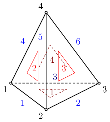
Fig. 14 LTRSpace element. Definition and node numbering convention.

Table 34 LTRSpace element summary

Keyword	LTRSpace
Description	Linear tetrahedra element
Parameters	NIP: allows to set the number of integration points (possible completions are 1, 8 (default), or 27).
Unknowns	Three dofs (u-displacement, v-displacement, w-displacement) are required in each node.
Approximation	Linear approximation of displacements and geometry using linear volume coordinates.
Integration	Full integration of all strain components using four point Gauss integration formula.
Features	Adaptivity support, Geometric nonlinearity support.
CS properties
Loads	Surface and Edge loadings supported.
Nlgeo	0,1,2.
Status	Reliable
Tests/Examples	sm/con2dpm9.in, sm/con2dpm10.in, sm/con2dpm11.in, sm/con2dpm12.in, sm/con2dpm6.in, sm/con2dpm7.in, sm/con1dpm1.in, sm/con1dpm3.in, sm/con2dpm1.in, sm/con2dpm2.in (and 15 more)

QTRSpace element

Implementation of tetrahedra ten-node finite element. Each node has 3 degrees of freedom. The element features are summarized in Table 35. Following node numbering convention is adopted (see also Fig. QTRSpace element. Definition and node numbering convention.):

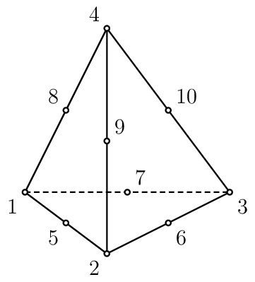
Fig. 15 QTRSpace element. Definition and node numbering convention.

Table 35 QTRSpace element summary

Keyword	QTRSpace
Description	3D tetrahedra element with quadratic interpolation
Specific parameters	[NIP (in)]
Parameters	NIP: allows to alter the default integration formula (possible completions are 1, 4 (default), 5, 11, 15, 24, and 45 point intergartion formulas).
Unknowns	Three dofs (u-displacement, v-displacement, w-displacement) are required in each node.
Approximation	Quadratic approximation of displacements and geometry using linear volume coordinates.
Integration	Full integration of all strain components using four point Gauss integration formula.
Features
CS properties
Loads
Nlgeo	0,1,2.
Status	Reliable

LWedge element

Implementation of wedge six-node finite element. Each node has 3 degrees of freedom. The element features are summarized in Table 36. Following node numbering convention is adopted (see also Fig. LWedge element. Node numbering convention in black, edge numbering in blue and face numbering in red.):

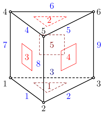
Fig. 16 LWedge element. Node numbering convention in black, edge numbering in blue and face numbering in red.

Table 36 LWedge element summary

Keyword	LWedge
Description	3D wedge six-node finite element with linear interpolation
Specific parameters	[NIP (in)]
Parameters	NIP: allows to alter the default integration formula (possible completions are 2 (default) and 9 point integration formulas).
Unknowns	Three dofs (u-displacement, v-displacement, w-displacement) are required in each node.
Approximation	Linear approximation of displacements and geometry.
Integration	Full integration of all strain components using four point Gauss integration formula.
Features	Layered cross section support.
CS properties
Loads
Nlgeo	0,1,2.
Status	Reliable

QWedge element

Implementation of wedge fifteen-node finite element. Each node has 3 degrees of freedom. The element features are summarized in Table 37. Following node numbering convention is adopted (see also Fig. QWedge element. Node numbering convention in black, edge numbering in blue and face numbering in red.):

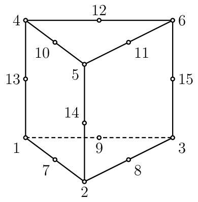
Fig. 17 QWedge element. Node numbering convention in black, edge numbering in blue and face numbering in red.

Table 37 QWedge element summary

Keyword	QWedge
Description	3D wedge six-node finite element with quadratic interpolation
Specific parameters	[NIP (in)]
Parameters	NIP: allows to alter the default integration formula (possible completions are 2 (default) and 9 point integration formulas).
Unknowns	Three dofs (u-displacement, v-displacement, w-displacement) are required in each node.
Approximation	Quadratic approximation of displacements and geometry.
Integration	Full integration of all strain components using four point Gauss integration formula.
Features	Layered cross section support.
CS properties
Loads
Nlgeo	0,1,2.
Status	Reliable
Tests/Examples	sm/qwedge_01.in

Layer stacking sequence definition for 3D elements

Selected 3D elements (bricks and wedge geometries) support using the LayeredCrossSection model to define layer stack as a sequence of individual layers. Individual layers are assumed to lie in element parametric \(\xi-\eta\) plane and are stacked along parametric \(\zeta\) coordinate of the element. The direction of parametric coordinates is determined by element node numbering convention, see figures with element geometries above. Note, that the stacking direction is in general the function of element geometry.

It is important to understand concept of element and material coordinate systems.

The element coordinate system (elemCS) coincides, by default, with the global coordinate system. The user-defined element coordinate system can be defined using lcs parameter. The lcs parameter defines an array of size 6, where the first 3 components define direction of local element-axis and remaining 3 components define direction of local element y-axis. The local element z axis is computed using vector product \(e_z=e_x\times e_y\).

The material properties of each layer are defined in material coordinate system (matCS). Also the solver output for individual layers is done in matCS. By default, the material coordinate system coincides with global coordinate system. Additionally, the material coordinate system for individual layer can be rotated around material CS z-axis by angle, defined by layered cross section rotations keyword. This array parameter allows to define rotation angle for individual layers and should be defined in degrees not radians. If matcs element keyword is present, but no lcs element record is defined, then the following definition of elemCS is assumed: \(e_x=\{\frac{dx(\xi,\eta,\zeta)}{d\xi},\frac{dy(\xi,\eta,\zeta)}{d\xi},\frac{dz(\xi,\eta,\zeta)}{d\xi}\}, h=\{\frac{dx(\xi,\eta,\zeta)}{d\eta},\frac{dy(\xi,\eta,\zeta)}{d\eta},\frac{dz(\xi,\eta,\zeta)}{d\eta}\}, e_z=e_x\times h, e_y=e_z\times e_x\), where \(\xi,\eta,\zeta\) are parametric element coordinates. The strains and stresses in individual layers are always reported in material coordinate system. LayeredCS integration The layered cross section integration can be set up using number of integrations points in layer plane (nintegrationpoints parameter ) and using number of integration points per layer thickness (layerintegrationpoints parameter).