Coupling mechanics and flow on a lattice — a swelling inclusion drives the pore pressure
The companion post drove the wall from the fluid. This one runs the coupling the other way: a stiff inclusion with a swelling interface deforms the surrounding matrix, the deformation generates pore pressure on the transport lattice, and through Biot's effective stress that pressure feeds back to thicken the matrix — reproducing both the logarithmic pressure field and the poroelastic displacement.
The previous post coupled the mechanical lattice (frame elements on the Delaunay edges) and the transport lattice (conduit elements on the dual Voronoi edges) in one direction: a prescribed fluid pressure deformed the solid. This post runs the coupling the other way — and then closes the loop.
A stiff inclusion with a swelling interface deforms the matrix; the deformation generates a pore pressure on the transport lattice (mechanical → transport); and through Biot’s effective stress that pressure feeds back into the matrix (transport → mechanical). It is the displacement-driven side of the same Grassl, Fahy, Gallipoli & Wheeler (2015) framework — the staggered scheme that, with cracking, becomes fluid-driven fracture.
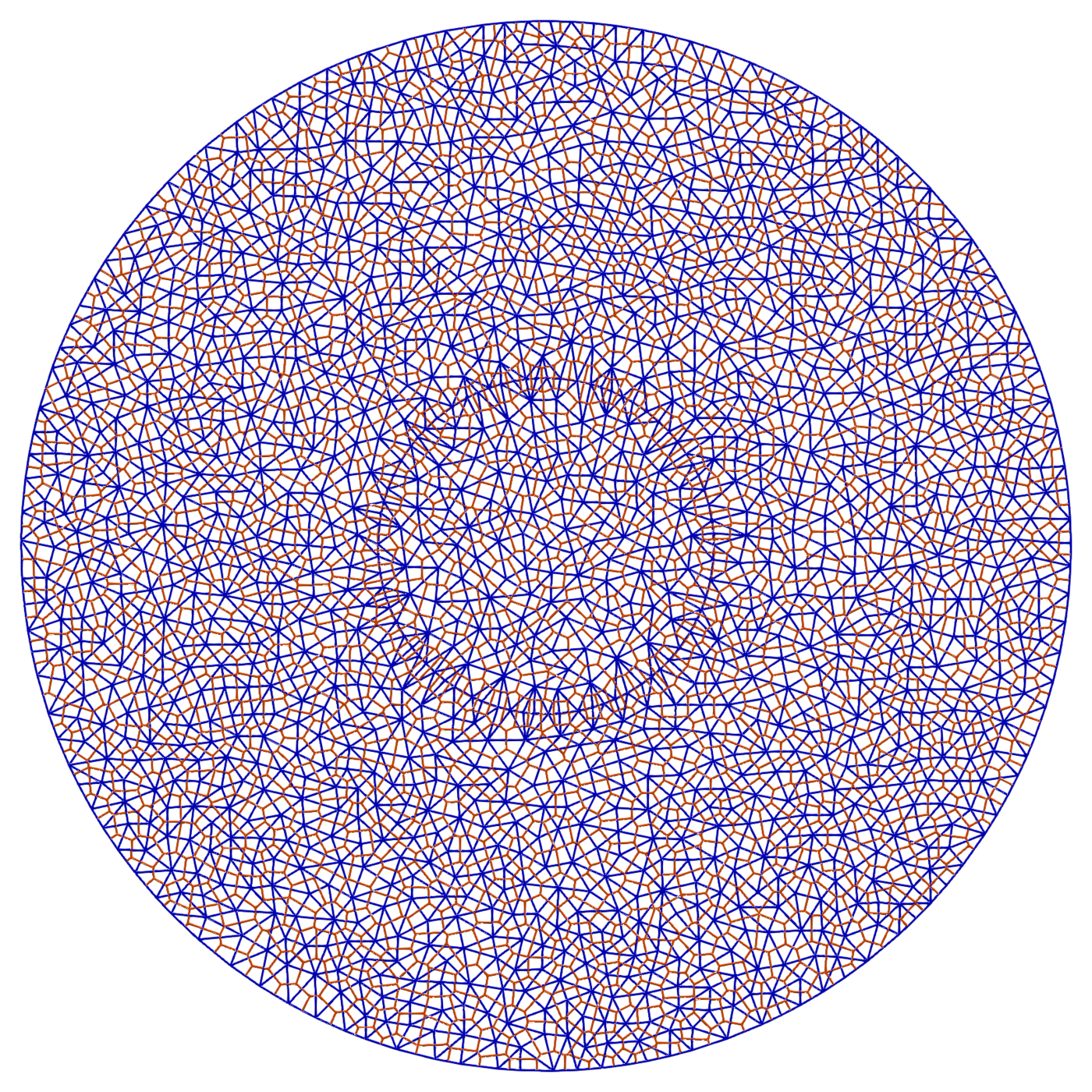
The dual lattice. Mechanical struts on the Delaunay edges (blue) and transport conduits on the dual Voronoi edges (orange) share one Voronoi–Delaunay mesh — the two sides of the coupling live on opposite sides of the duality.
The problem
A concrete matrix disk (radius b) holds a stiff circular steel
inclusion (radius r_i), separated by a thin interfacial transition zone
(ITZ). The ITZ expands radially — an eigen-displacement, the way a corroding
bar or a swelling aggregate pushes on its surroundings. Because the inclusion
is far stiffer than the matrix, that expansion acts like a prescribed radial
displacement on the inner edge of the matrix annulus a … b.
The expansion compresses the radial ITZ struts. That compressive axial stress is what drives the flow problem.
How the deformation drives the flow — and back
Mechanical → transport. Each transport node on the ITZ midline is fed the
axial stress of its two flanking radial ITZ elements (a
LatticeDirichletCoupling boundary condition: compression sets a pore
pressure there). With the outer boundary drained (P_f = 0) and zero
storage, the transport problem reaches steady state, so the pore pressure
follows the same logarithmic radial profile as the pressure post,
P_f(r) = P_a · ln(b / r) / ln(b / a_p),
high at the inclusion, zero at the rim — only now P_a is generated by the
deformation rather than prescribed.
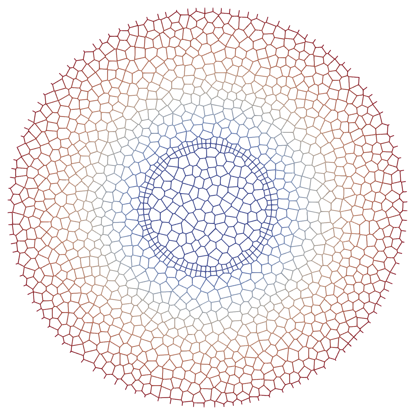
Pore pressure on the transport lattice — compressive (blue) at the swelling inclusion, draining to zero (red) at the rim.
Transport → mechanical. Total stress is effective stress plus a fraction of the pore pressure,
σ = σ_eff + b · P_f,
with b Biot’s coefficient. At b = 1 the pore pressure acts as a
distributed body force throughout the matrix; its gradient pushes the solid
outward everywhere. So the matrix carries both the inclusion’s inner
push and the fed-back pore pressure.
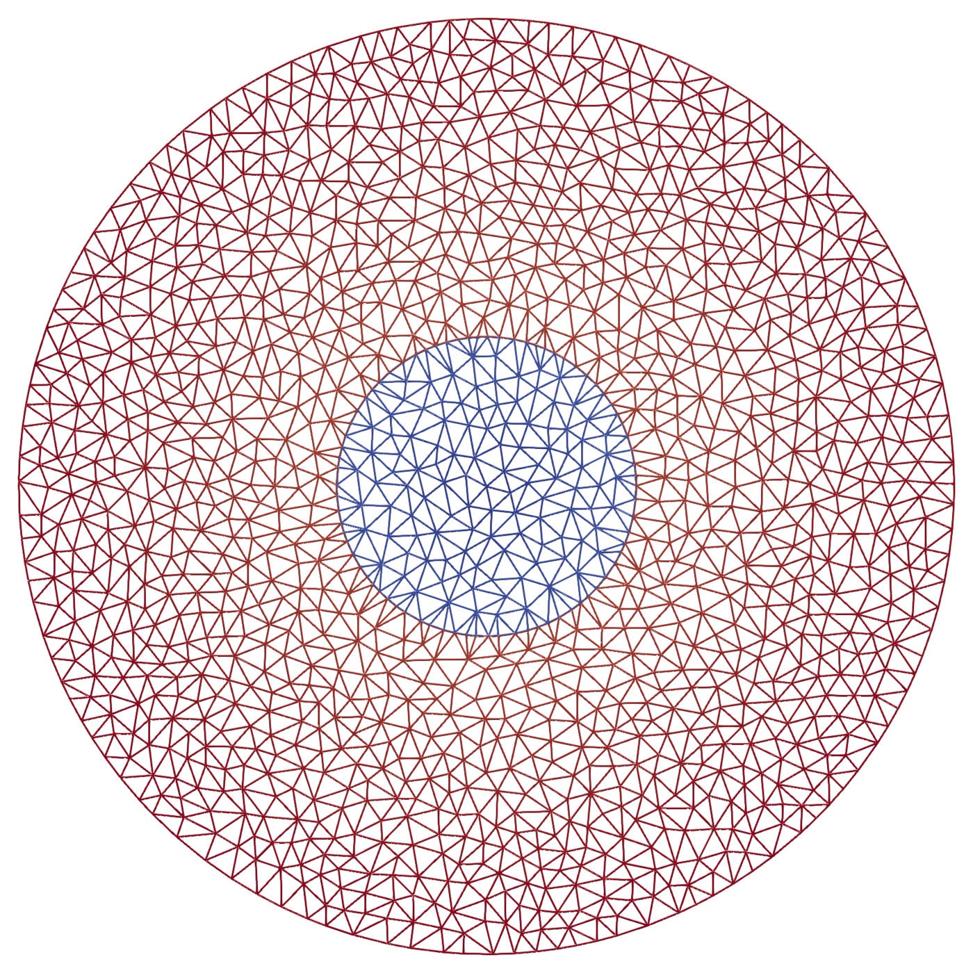
Radial displacement on the mechanical lattice — the stiff steel inclusion (blue) barely moves while the matrix (red) is pushed outward.
The two sub-problems are solved in a staggered loop — mechanics first (so the stress exists for the transport to read), then transport — exchanging stress and pressure each step.
Lattice vs analytical
The transferred pressure. The pore pressure on the transport lattice,
normalised by the ITZ-midline value P_a, against normalised radius
r / r_i — raw lattice nodes (scatter) against the logarithmic profile (line):
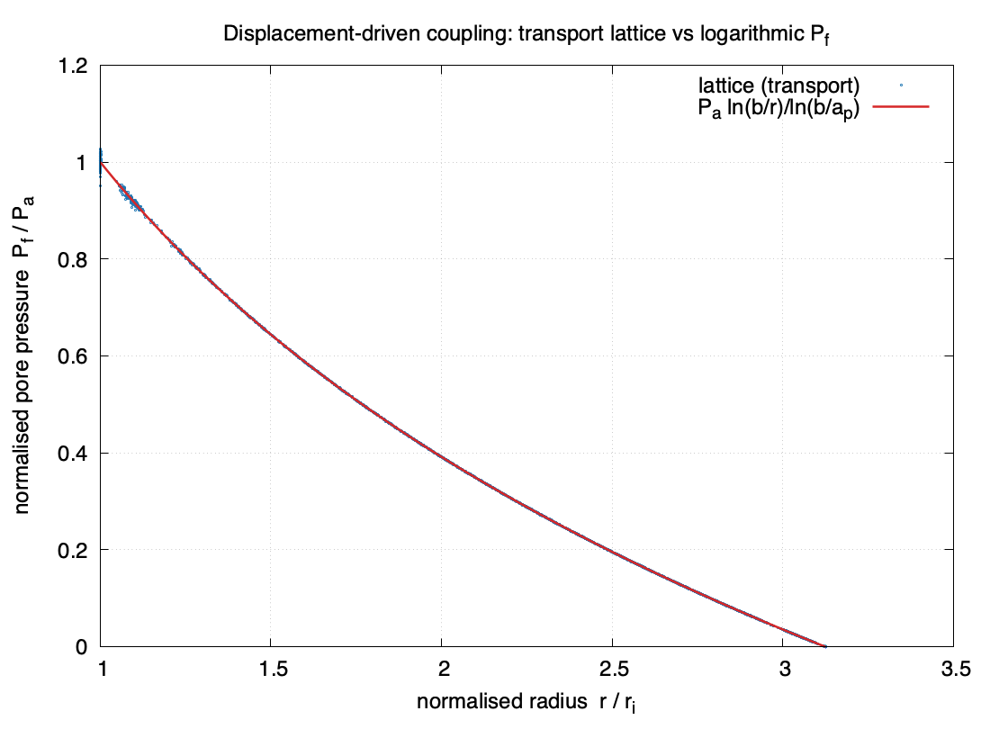
The deformation-generated field is logarithmic, just as a prescribed inner pressure would give — the coupling transfers the stress to the fluid cleanly.
The fed-back displacement. Here is the nice part: that same pore pressure
P_a is the ITZ axial stress, which is the radial traction the ITZ applies
to the matrix. So the matrix annulus is loaded by σ_r(a) = P_a at the inner
edge, a traction-free outer edge, and — because the matrix now carries the
distributed pore-pressure body force — the poroelastic solution
u_r(r) = (κ/2) r ln r + D r + C1/r with κ ∝ b · P_a. The displacement is
predicted from the computed pressure, with no fitted amplitude:
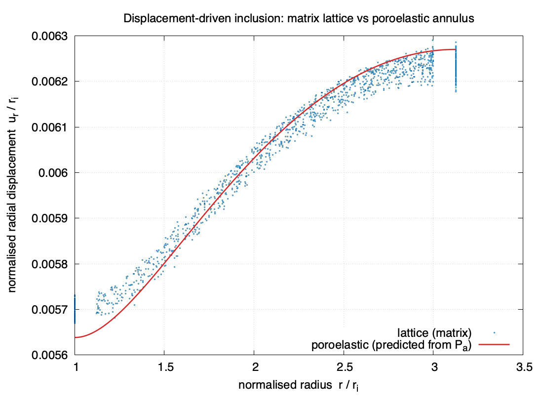
u_r increases with radius — the wall thickens. Without the feedback
(b = 0, κ = 0) the same load gives the Lamé result, where u_r decreases
and the wall thins. The Biot feedback flips it, exactly as the inner pressure
did in the previous post — reached here from the opposite direction.
This elastic case is the baseline. Let the ITZ keep expanding and the matrix crack, and the same coupled lattice — pore pressure on the Voronoi dual, effective stress on the Delaunay frame — drives the pressure-and-cracking problem of the 2015 paper, now from a deformation source.
Reproduce
git clone https://github.com/githubgrasp/oofem-examples.git
cd oofem-examples/lattice-coupling-displacement-2d
docker run --rm -v "$PWD":/work ghcr.io/githubgrasp/oofem-public:lattice-coupling-displacement-2d bash run.sh
The converter writes both subproblems from one shared mesh (#@grid 2dSMTM);
run.sh solves the staggered problem and draws pressure.png and
displacement.png. Setting bio 0.0 in control.in (and dropping
#@couplingflag) switches off the feedback and recovers the Lamé thinning —
compare.py swaps the analytical curve automatically. The run takes about
fifteen seconds.
The :lattice-coupling-displacement-2d image tag is immutable — use :latest
instead to track the current OOFEM build (results may drift slightly as the
code evolves).
Built with OOFEM.